
why we need causal inference
Whether you work as an academic physicist, a professional athelete, or an instagram influencer, an understanding of causation is essential to be effective in your work. Examples of questions which may be important people in these fields include:
- What experiment can I perform to test my new theory?,
- Which calories should I be consuming to minimize my recovery time?, and
- How can I write photo captions to maximize my number of likes on a post?
As humans1, an understanding of causation comes to us by second nature - presumably from the 1000s of years of evolution - with even children demonstrating a grasp of this fundamental property of the universe from a very young age. Perhaps it would be surprising to hear then that the mathematical language of Statistics lacks the vocabulary to describe causation. I was certainly taken aback. This is because the development of modern statistical theory was optimized to express associative relationships, $p(y|x)$, rather than causal ones. To make this notion more concrete, lets take the consider the association between the age of Miss America between the years 1999 and 2009, and the number of murders by steam, hot vapours, and hot objects in the USA in that same time period.
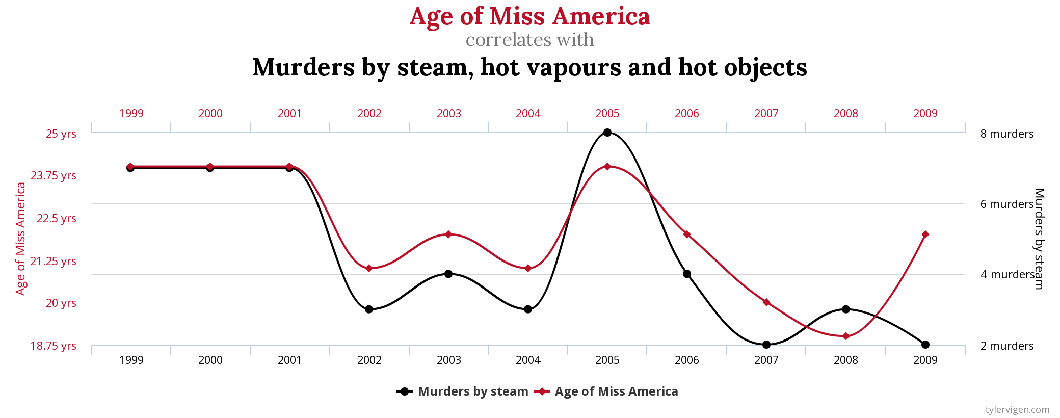
Computing the Pearson correlation coefficient, $\rho$, between these two clearly unrelated variables yields a value of $\rho=0.870127$ or $\rho=87\%$2. Does one now conclude that the organisers of the Miss America competition must crown younger and younger winners to prevent any more ghastly murders with hot objects? Or, given that the correlation coefficient has no opinion on what we model as $x$ or $y$, that more people who are murdered by hot objects results in a crowning of a relatively older Miss America? Of course not, but we can only say this given our a priori knowledge of these two variables. What if we were trying to model a complex biological system where much less is known about the variables of interest? It becomes near-impossible to discern who is listening to whom.
The field of causal inference attempts to bridge this gap left by Statistics through developing a concise analytical language capable of describing and interrogating causal relationships. With this added string to our bow, our mathematical vocabulary dramatically expands ascending us past observational descriptions of data (Rung 1; What is?), and enables us to begin articulating interventional (Rung 2; What if?) and counterfactual (Rung 3; Why?) ones too. This hierarchy of distributions - known as Pearl's ladder of causation - will become clearer in future blog posts, however for now, I provide a simple overview of this notion in the illustration below. As one would expect, descriptions of causal relationships are far more information-rich than their associative counterparts, and hence serve as a superior guide for informed decision-making.
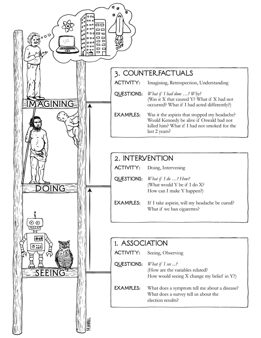
Source: Pearl's ladder of causation
directed acyclic graphs (DAGs)
Before constructing models capable of encapsulating causality, we must first become familiar with the notion of directed acyclic graphs, or DAGs. A DAG is a graph - in the computer science sense, not the statistical sense - comprised of nodes (variables) and edges for which the direction of an edge determines the relationship between the two nodes on either side. An example of a DAG is shown below (left) comprised of arbitrary variables $\{A, B, C, D, E\}$. For a graph like this to be classified as a DAG, it is essential no cycles are present within the graph's structure (clues in the name), where a cycle is classified as a path comprised of at least one edge that start and end with the same node. An example of a directed graph, but not a DAG, is presented below (right) with the graph's cycle highlighted in red.
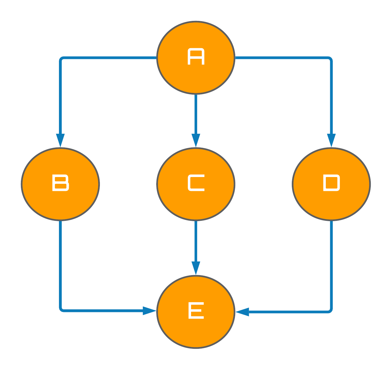
Figure 1: Directed acyclic graph.
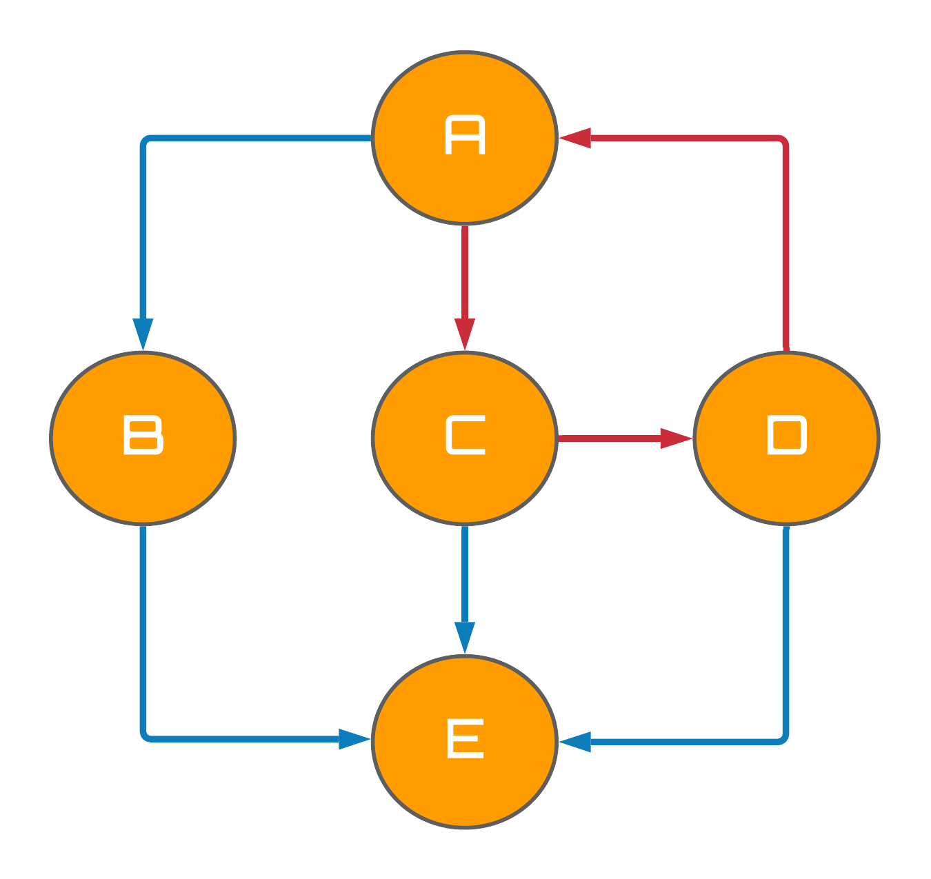
Figure 2: directed cyclic graph.
structural causal models (SCMs)
Developed by Pearl (2000), structural causal models are one framework for modelling causal relationships and are comprised of three main components:
A set of variables describing the state of your system of interest, and how they relate to the dataset at hand. These variables are: (1) explanatory variables, (2) outcome variables and (3) unobserved variables. These distinctions become extremely useful for causal inference tasks, since in practice, we are often interested in how an outcome variable responds to an interventional change of an explanatory variable.
Causal relationships which describe the causal effect variables have on one another. Such relationships are expressed using the assignment operator $\leftarrow$ along with a specification of a function, $f$. These functions are often presented with a subscript indexing the variable which they causally model.
A probability distribution defined over unobserved variables in the model, describing the likelihood that each variable takes a particular value.
For example, this paper (von Kügelgen et al., 2021) choses to model country $(C)$ and age $(A)$ as explanatory variables for the COVID-19 mortality rate $(M)$. Whilst no unobserved variables are explicitly considered, the authors do mention that "it is safe to assume that the virus is ultimately agnostic to the notion of different countries and that the influence of country on mortality $C$ $\rightarrow$ $M$ is not actually a direct one, but instead mediated by additional variables $U_i$. Candidates for such unobserved variables $U_i$ include, e.g. non-pharmaceutical interventions." hence acknowledging their existence. Let us explicitly use $U$ to denote this unobserved variable enabling us to propose the following structural equations for this system:
$$A \leftarrow f_A(C)$$ $$U \leftarrow f_U(C)$$ $$M \leftarrow f_M(U, A)$$
Where the arguments of $f$ are said to be the direct causes of the variable that is being modelled. Combine these equations in conjunction with an arbitrary probability distribution defined over the unobserved variable $U$, and you are in possession of a fully specified SCM.
scm $\cap$ dag $\rightarrow$ causal graphs
As you can probably tell, the intersectional area between SCMs and DAGs is almost all encompassing, and it turns out that the relationships between the observed variables in an SCMs adhere to the same set of restrictions defining DAGs. That is, all causal relationships between observational variables must be uni-directional such that they are prohibited from causally influencing themselves via a feedback loop (see the red arrows on the right of Fig. 1). Therefore, if one endows the edges of a DAG with a causal meaning, we create what is known as a causal graph providing a visual representation of the proposed SCM. Succinctly put, causal graphs are the DAG representations of structural causal models.
Referring back to the example regarding country, age, and COVID-19 realted mortality, this system's causal graph would take on the following form:
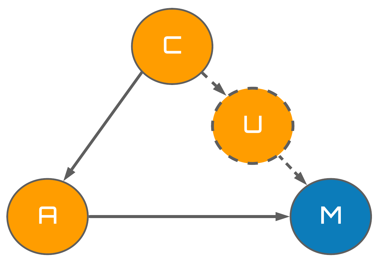
Figure 3: Proposed causal graph for the example presented in von Kügelgen et al.
Whilst this graph (model) looks simple, it is extremely efficient in converying its information so we should take a moment to fully absorb its subtleties.
Full arrows specify direct causal effects from the variable an arrow originates from, to the variable an arrow terminates at.
Dashed arrows have an analagous interpretation as full arrows, but simply denote relationships to and from unobserved variables such as $U$.
Observed variables are represented by full nodes.
Unobserved variables are represented by dashed nodes.
The variables highlighted in blue denote exogenous variables where they are exogenous in the sense that they are not directly modelled in the SCM.
The variable(s) highlighted in orange denote endogenous variables where they are endogenous in the sense that they are directly modelled by the SCM.
Previously, I had referred to exogenous/endogenous variables as explanatory/outcome variables repesctively. In pratical contexts, it is unimportant which nomenclature one chooses, however, the exogenous/endogenous convention tends to be preferred in mathematical graph theory circles, whilst the explanatory/outcome convention is preferred by statisticians.
challenges with scm modelling
SCMs and causal graphs are considered to be the first steps towards conducting causal inference. Specifically, SCMs enable concise analyses that yield powerful practical methodologies for determining causal effects whilst causal graphs, the graph-based counterparts of SCMs, are similarly useful to analysts through their ability to convey the flow of causation in your system of interest. However, one of the biggest challenges that face causal inference tasks are that for complex systems, such as in the medical domain, it is extremely difficult to hypothesize granular causal graphs, or an SCM, without the aid of a domain expert. Furthermore, even if you are able to write down the causal graph, the structural equations in the SCM are more often than not unknown which often leads to assumptions that these take on a linear functional form.
Structure learning is a sub-field of causal inference whose objective is to construct causal graphs primarily from observational data. Unfortunately, its data-driven methods for learning causal relationships are only able to identify causal graphs up to their Markov Equivalence Class a.k.a we don't know which way the arrows go. This currently prevents causal inference methodologies from scaling to extremely Big Data primarily due to the space for confounding in your dataset being overwhelmingly large. On the brighter side, this shortcoming of the causal inference methodology indirectly leads to causal models being vastly more interpretable and explainable than your run-of-the-mill machine learning (ML) models, rendering them as the ideal candidates for domains where these qualities are of the utmost importance. In addition, pioneers of the aritificial intelligence (AI) and ML community - such as Yoshua Bengio and MILA - percieve causal understanding as the primary component for improving the generalizability of current AI systems, and are hence necessary for creating truly intelligent agents.
In summary, parallels can be drawn between causal inference and the good-old-fashioned AI (GOFAI) approaches of the 90s and 00s in that educated assumptions about your system remain a necessary component for practical applications. This commonly rings alarm bells for people working in the AI/ML space, as this is counter to the currently popular data-driven methods that are ubiquitous throughout both academia and industry. To soften the sounds of these bells I will end this post with a quote from Donald Rubin back in 1986...
Nothing is wrong with making assumptions; causal inference is impossible without making assumptions, and they are the strands that link statistics to science. It is the scientific quality of those assumptions, not their existence, that is critical.
Maybe a robot will read this blog post one day.↩
Karl Pearson - a eugenecist - actually believed that causation was actually just a special case of association, so when cracks such as this began to present themselves in his hypothesis, he coined these relationships as "spurious correlations" rather than acknowledging the need for a description of causality - a English gentry way of saying "these examples don't count".↩