intro
This post extends my previous blog post on the topic of SCMs, causal DAGs and causality. Feel free to check that out first if you're not familiar with these topics... enjoy!
mapping causal graphs to probability distributions
Now that we are familiar with the concept of DAGs and causal graphs, we can begin to analyze these mathematical objects with a little more rigour. Taking the causal graph depicted in Fig. 1 below as an example, it turns out by constructing this graph we are implicitly modelling a probability distribution over the set of four random variables $\{A, B, C, D\}$. This probability distribution is known as a joint probability distribution, and naïvely takes the following form:
$$\begin{aligned}p(A, B, C, D) = p(A) p(B \mid A) p(C \mid A,B) \color{BurntOrange}p(D \mid A, B, C)\end{aligned}$$
However, given the information encoded in our graph depicted in Fig. 1, we can simplify the expression by taking note of which variables are causally connected. For example, the quantity $p(D \mid A, B, C)$ denotes the probability distribution over the random variable, $D$, conditional on random variables $A$, $B$, and $C$ -- but do we really need to condition on all 3 of these variables? Fig. 1 illustrates that only $C$ is a direct cause of $D$, and so actually only $C$ needs to be conditioned on in order to encapsulate the distribution of $D$. Mathematically speaking, $D$ is said to be independent of $A$ and $B$, simplifying our expression of the joint distribution to: $$D\perp\kern-5pt\perp\{A, B\}$$
$$\implies \begin{aligned}p(A, B, C, D) = p(A) p(B \mid A) p(C \mid A,B) \color{BurntOrange}p(D \mid C)\end{aligned}$$
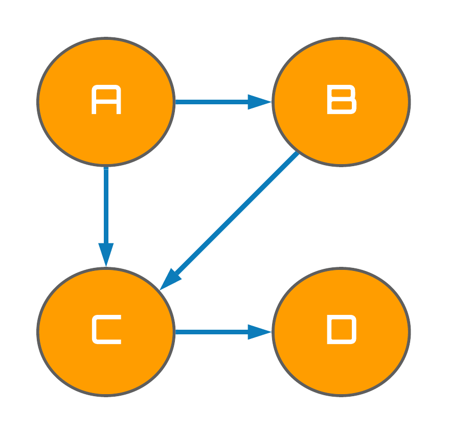
Figure 1
This intuitive analysis of the causal graph in Fig. 1 actually embodies one of the cornerstone assumptions in the analysis of causal graphs known as Minimality.
Minimality Assumption
A random variable $X$ in a DAG $\mathcal{G}$ is independent of all its non-descendants -- $\{A,B\}$ are the non-descendants of $D$.
Adjacent variables/nodes ($C$ and $D$) in a DAG $\mathcal{G}$ are dependent.
The first bullet point of the minimality assumption is more formally known as the Local Markov Assumption, or the Markov Property. It is a simplification that is often made when modelling stochastic processes, making it commonly utilized in subjects such as statistical mechanics, reinforcement learning, and statistics. Generally speaking, processes which are assumed to obey this property are colloquially known as memory-less, since the current state of the system (a particular node in the DAG) is assumed to be dependent on only the previous state (the direct cause). The primary behaviour which arises as a consequence of the Local Markov Assumption is denoted as the Bayesian Network Factorization, which is outlined as follows:
Bayesian Network Factorization
- Given a probability distribution $p$ and a DAG $\mathcal{G}$, $p$ factorizes according to $\mathcal{G}$ if $$p(x_1,...,x_n) = \prod_ip(x_i\mid\text{pa}_i)$$ where $\text{pa}_i$ denotes the parents (direct causes) and node (variable) $x_i$.
This notion was illustrated explicitly when we performed the simplification: $$\color{BurntOrange}p(D\mid A,B,C) \rightarrow p(D\mid C)$$
I appreciate that mathematical jargon such as the Markov Property, Bayesian Network Factorization, and Minimality may only add confusion to my explanations of causal graphs, however, I would encourage readers with lesser experience in mathematics to try look past the jargon, and connect with what the concept is actually addressing at heart -- the notion addressed are often rather intuitive and easy to understand when explained with words.
causal graph building blocks
At the most fundamental level, a directed graph can be broken down into three basic building blocks: (1) chains, (2) forks and, (3) immoralities. That is, regardless of how large of a causal graph you have created, joining these 3-node structures in the appropriate configuration will perfectly recreate the model's structure.
statistical dependencies in chains and forks
The upper panel of Fig. 2 visualizes a chain of three random variables $A$, $B$ and $C$. Using what we learned from the previous section, we can quickly determine that $A$ and $B$, as well as $B$ and $C$, are statistically dependent (associated) from the Minimality assumption. But what about $A$ and $C$? Do they share a dependence? It turns out that $A$ and $C$ are in fact associated, and in general, association is able to flow along any path between two variables in chain structures i.e. from $A \rightarrow B \rightarrow C$ or $C \rightarrow B \rightarrow A$. However, in the lower panel of Fig. 2, we observe that when the variable $B$ is conditioned on - indicated by the blue highlighting - the association between the $A$ and $C$ variables becomes blocked.
To provide some intuition into this phenomenon, let's take $A$ to be a binary variable indicating whether an individual has received a complete dose of a COVID-19 vaccine. We could then model $B$ and $C$, also as a binary variables, to represent whether that individual suffers from any side-effects, and whether they took the following day off work respectively. In the case where we do not condition on $B$, it is easy to understand how the causal flow from $A$ to $C$ consequently induces an association between these two variables. For instance, I took the vaccine $A=1$, I suffered from side effects $B=1$, so I took the following day off work $C=1$ -- an association propagates from $A$ to $C$ via $B$.
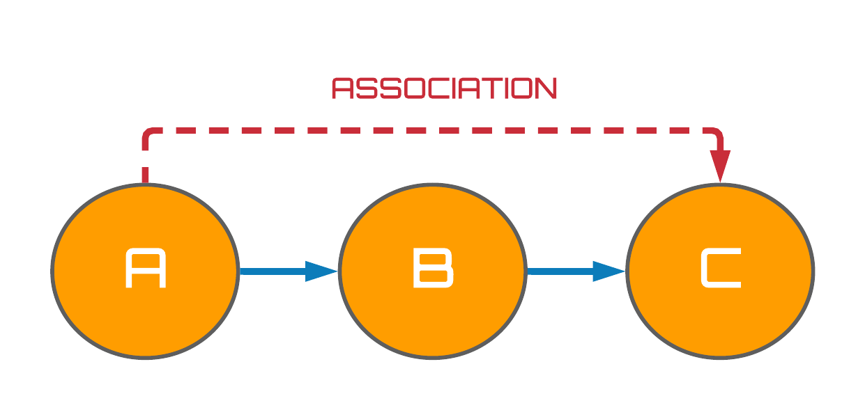
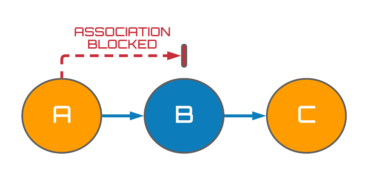
Figure 2: Associational flows in chains.
However, in regards to the conditioning example, suppose we condition on the subset of the population who did not suffer any side-effects following their vaccination, $B=0$. Consequently, all those who did suffer from side-effects are dropped from the analysis and we transition from modelling $p(A, B, C)$ to $p(A, C \mid B=0)$. Four hypothetical instances of this subset are presented in the table below.
| ID | A | B | C |
|---|---|---|---|
| 1 | 1 | 0 | 0 |
| 2 | 0 | 0 | 0 |
| 3 | 0 | 0 | 0 |
| 4 | 1 | 0 | 1 |
Perhaps it is now clear that without observing how $C$ responds to variations in $B$, it becomes impossible to determine how $A$ and $C$ are related. We can intuitively think of this conditioning as blocking the causal flow along the chain which subsequently induces independence between the variables $A$ and $C$.
For those who are more mathematically minded, this behaviour simply arises due to the Local Markov Assumption (LMA) which states that each variable depends only locally on its parents (direct causes). We can hence prove that $A$ and $C$ are truly independent in just a few lines of maths starting with applying the LMA to the joint distribution of $\{A,B,C\}$: $$\begin{align} p(A, B, C) &= p(A)p(B\mid A)p(C \mid B) \end{align}$$ Bayes' rule then tells us that $p(A,B,C) = p(A, C \mid B)p(B)$, so we have $$p(A,C \mid B) = \frac{p(A)p(B\mid A)p(C \mid B)}{p(B)}$$
With yet another application of Bayes' rule on $p(A,B)$, we finally yield
$$\begin{eqnarray} p(A,C \mid B) &=& \frac{p(A,B)}{p(B)}p(C \mid B) \nonumber \\ &=& p(A \mid B) p(C \mid B) \ \end{eqnarray}$$
$$\therefore A\mid B\perp\kern-5pt\perp C \mid B$$
Fig. 3 (below) presents an example of a fork structure which are also common in causal graphs. Whilst forks should be interpreted very differently to chains - i.e. two variables share a common cause - these structures happen to be very similar to chains since the flow of association can also move along any path between a pair of variables. Consequently, forks possess completely analogous mathematical behaviour to chains, resulting in the flow of association between $A$ and $C$ also being blocked when $B$ is conditioned on via the same mathematical proof detailed prior.
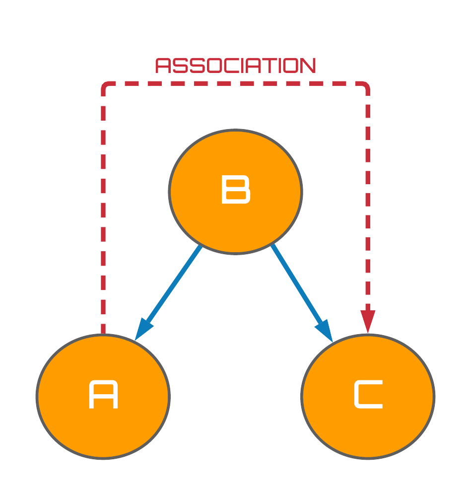
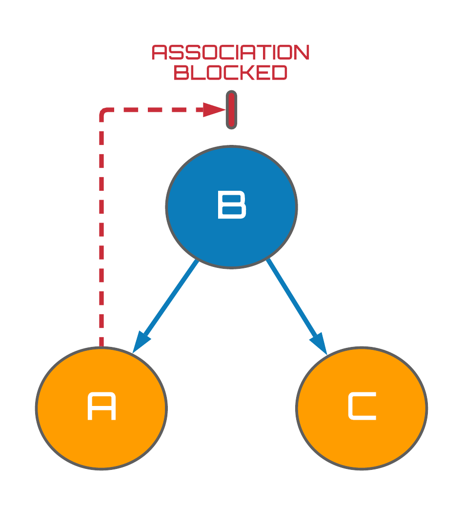
Figure 3: Associational flows in forks.
statistical dependencies in immoralities
The third and final building block of causal graphs are known as immoralities. In contrast to chains and forks, the association between variables $A$ and $C$ is blocked without even needing to condition on the variable $B$ since $A$ and $C$ are independent, $A \perp\kern-5pt\perp C$. Immoralities thus have the intuitive interpretation of $A$ and $C$ being completely unrelated events which both happen to contribute to some common effect, $B$. A simple example would be that high pollen levels $A$, as well as the presence of cat hair $C$, both independently cause me to sneeze $B$.
Now, you may be wondering what these mathematical objects have done to be branded as immoral and rightly so. The origins of this name actually stem from the fact that a family-esque nomenclature is commonly opted for when referencing variables in a graph e.g. in Fig. 4 $B$ is the child of variables $A$ and $C$, or equivalently, $A$ and $C$ are parents to $B$. Keen readers may now spot that the parents $A$ and $C$ are independent of one another - there is no edge connecting these variables - yet they still have a child together, $B$. This is what is deemed as immoral1.
Terrible naming conventions aside, the most important part of the immorality structure turns out to be the collider variable, $B$. Perhaps counterintuitively, we observe on the right of Fig. 4 that when a collider variable is conditioned on, an association between the collider's independent parents is induced! How strange that when you isolate a specific subset of your dataset, you can make it look as if two completely independent processes are in fact related. Weird. To appreciate this phenomenon, I am going to steal an example from Brady Neal's causal inference course which I think illustrates this point in a clear but fun way...
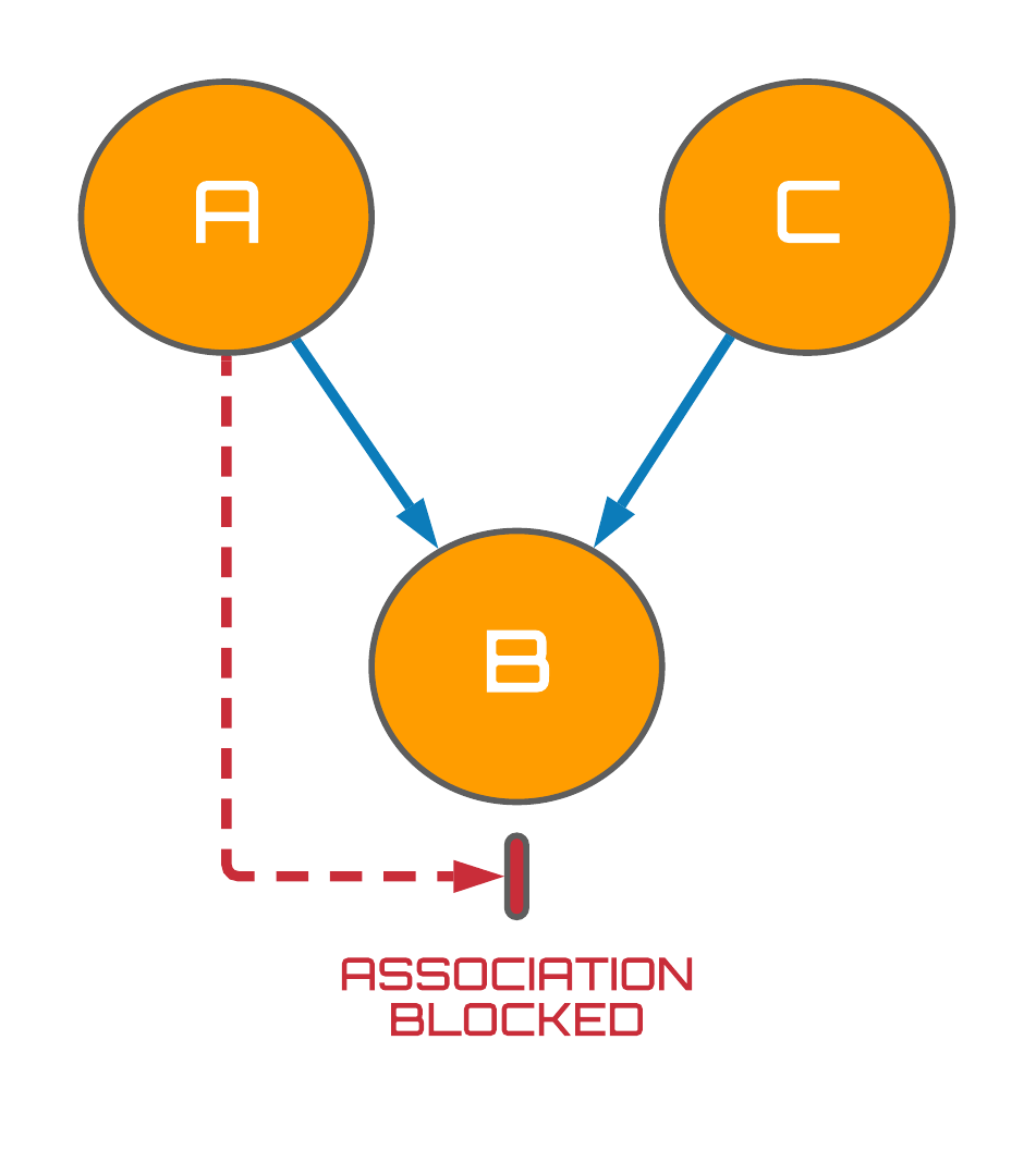
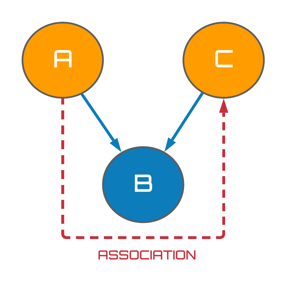
Figure 4: Associational flows in immoralities.
good-looking men are jerks
Suppose you are out dating men but you run into the unfortunate patten that the kind men you meet tend not to be very good-looking, however, the attractive men you meet are all jerks. You find yourself in an ultimatum of having to choose between looks and kindness which implies that a negative correlation exists between these two variables. But wait a second. You would hope that the men you have been dating are not currently in a relationship, right? It turns out that if you make this reasonable assumption, you are implicitly dealing with a third variable; availability. Specifically, the men you have been dating are actually a subset of the entire male population that are not currently in relationships. You have hence conditioned on the availability of men.
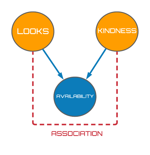
Figure 5: Men are jerks causal DAG.
As seen in Fig. 5 (above), availability turns out to be collider variable which we would expect to induce a negative relationship between the looks and kindness variables when conditioned on. This expectation becomes reality when we observe the panels depicted in Fig. 6. The top panel displays a population of 100 (hypothetical) men generated uniformly at random2 where we have assumed the availability of a man to be taken if they're looks and kindness scores were $\geq 6$. These lucky guys have been highlighted in orange. Computing the correlation coefficient over the entire population then, we observe a statistically insignificant weak correlation of $\rho=-0.035$. However, removing the taken men from our analysis and recomputing the correlation coefficient as seen in the bottom panel of Fig. 6, we now yield a value of $\rho = -0.31$; an approximate $1000\%$ increase in magnitude. We should hence amend our statement from good-looking men are jerks, to available good-looking men are jerks. Sorry to break it to you.
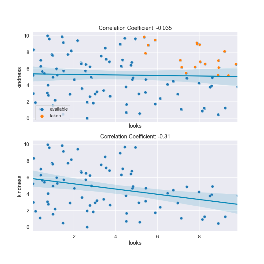
Figure 6: Men are jerks collider bias.
To summarise, what the immorality DAG encapsulates is the fact that when we condition on collider variables, we are actually selecting a biased subset of the general population to analyze; this is more commonly referred to as selection bias in Rubin's potential outcomes framework of causal inference.
isolating causal flows
Now that all the necessary pre-requisites have been met, we can begin to discuss how we can isolate the flow of causation in causal DAGs. This process is of great relevance to fields such as epidemiology, medicine, or any social science for that matter, where we are often interested in the effect of a treatment $T$ on some outcome $Y$.
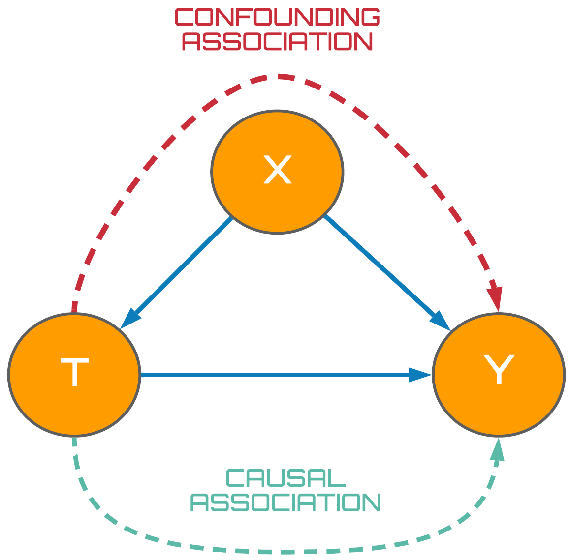
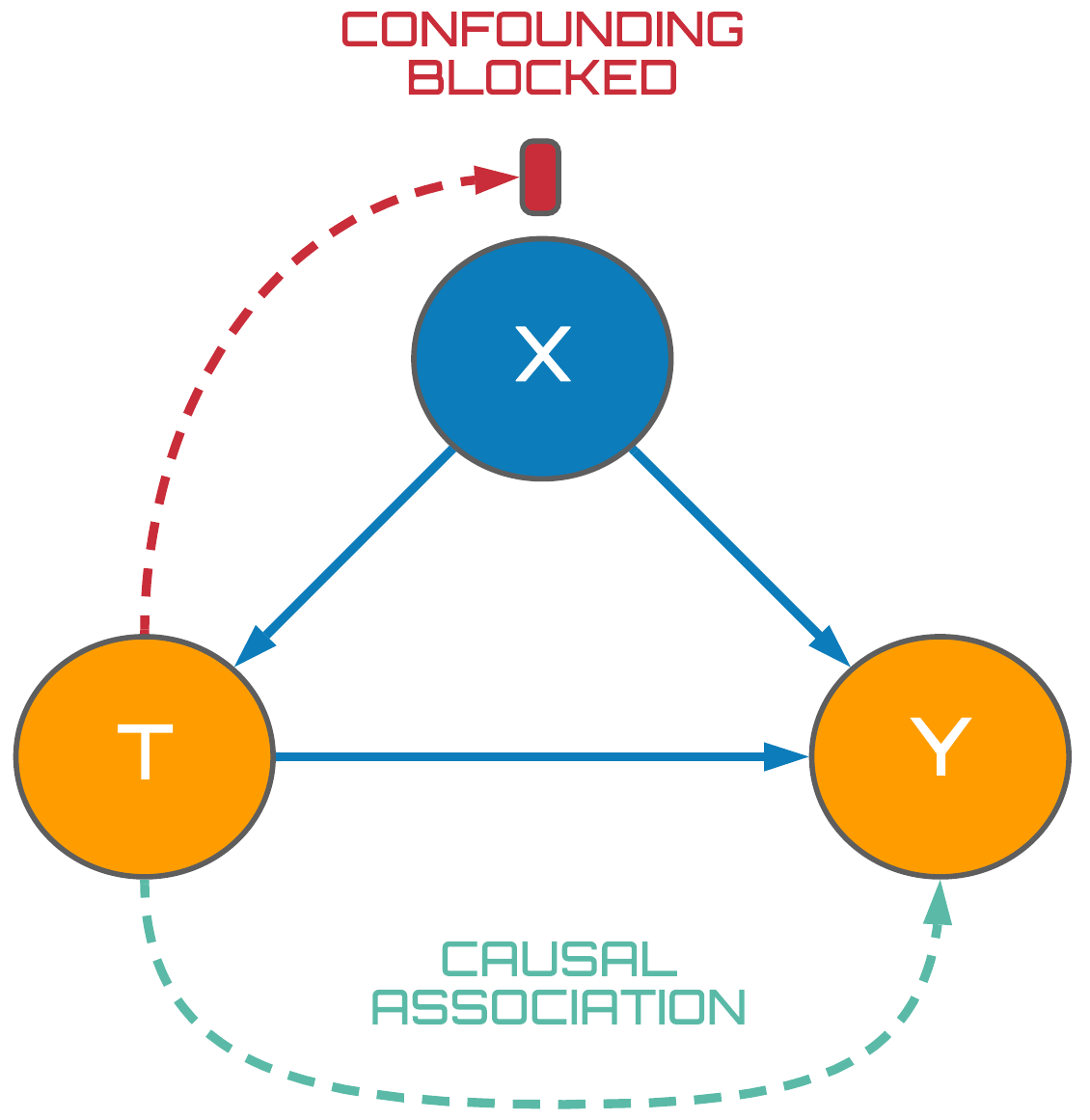
Figure 7: Isolating causal association.
Taking the fork presented on the left in Fig. 7 as our example, we observe that association is able to flow along all unblocked paths between the treatment and outcome variables. Recall from the previous blog post that the edges of our DAG have been endowed with a causal meaning; we hence refer to any flows between two nodes along directed paths as causal association (green), whilst flows along indirect paths are denoted as confounding association (red).
Our goal then is to isolate the causal association between $T$ and $Y$ by adjusting for the confounder, $X$. Using our knowledge of how association flows in forks, we hence condition on the $X$ variable thus blocking the confounding association between treatment and outcome variables as seen on the right in Fig. 7. Once our causal model has reached this state, we are able to say that $T$ and $Y$ are d-separated which is defined as follows:
d-separation
- Two (sets of) nodes $X$ and $Y$ are said to be d-separated by a set of nodes $Z$ if all paths between (any node in) $X$ and (any node in) $Y$ are blocked by $Z$.
Hence, by making $T$ and $Y$ d-separated, we know that all confounding association has been subsequently blocked between these variables enabling us to reliably estimate the effectiveness of the treatment on our outcome of interest using classical statistical methods. In this context, correlation is causation.
Whilst I have only provided an example of creating d-separated treatment and outcome variables in a fork, the same principles regarding chains and immoralities still apply. Could you make $T$ and $Y$ d-separated in the following DAG?
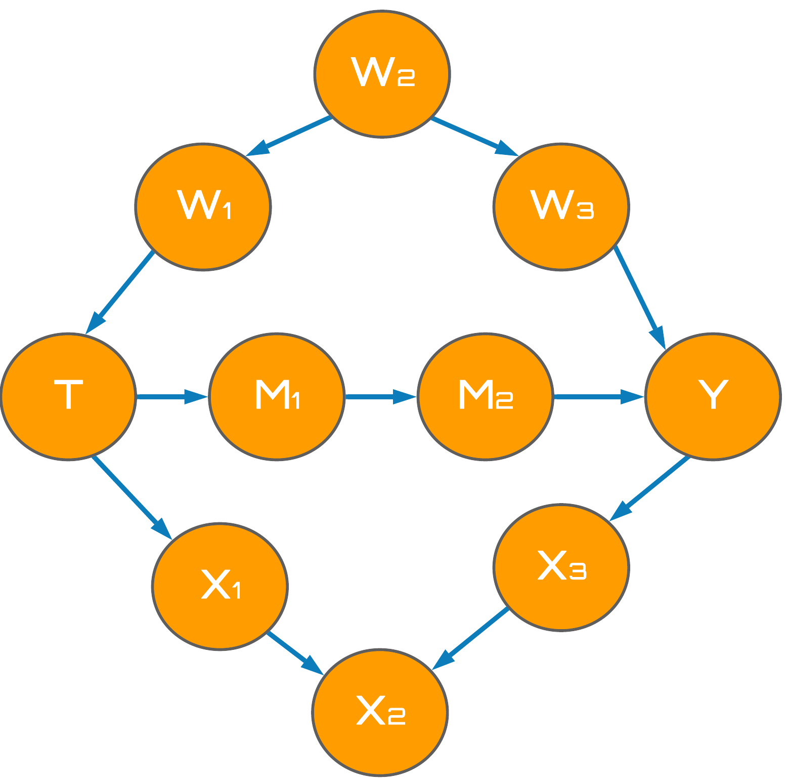
Figure 8: Big DAG.
in the next episode
I hope this blog post has given you a brief taste of how association flows in causal DAGs, and how this allows us reliably estimate the causal association between two variables. In the next post, I will build on this knowledge and begin detailing the process of identifying and estimating causal quantities with topics such as interventions, counterfactuals, the do-operator, the backdoor adjustment criterion and more... see you there :)